Every price makes a promise. When you buy a house, you pay today for value that arrives over decades. Built into that price is an expected growth rate. If the growth comes, the price was fair. If it doesn't, someone overpaid.
For most of the last decade, house prices kept their promises and then some. That has changed. Consumers still expect prices to grow about as fast as before. But the forces that drive long-run housing demand ares lowing. For lenders and investors, the gap between the promised growth rate and the likely one is a source of risk. That risk is not spread evenly. It is concentrated in particular places.
For a decade, prices beat expectations. Now they don't.
The New York Fed asks consumers every month how much they expect home prices to change. Compare each February's answer with what prices actually did over the next 12 months. From 2014 through 2024, prices beat the median expectation in ten of eleven years, often by a wide margin.
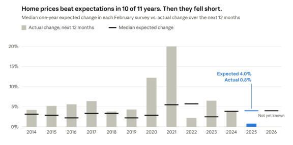
That pattern has flipped. In February 2025, the median consumer expected prices to rise 4.0% over the next year. The Case-Shiller national index rose 0.8%. Yet in February 2026, consumers still expected 4.0%. They also expected prices to rise about 3% a year over the next five years. Before 2020, that five-year figure was closer to 2 to 2.5%. The promise has grown, even as the last year failed to keep it.
Past gains are a poor guide
Where do growth expectations come from? Mostly from the past. Buyers look at what prices did over the last few years and extend the line.
But past gains mix two different things. One is real growth in demand: more households, and households with more income. That kind of growth can repeat. The other is a one-time jump, where buyers simply pay more for the same house. That kind cannot repeat on its own.
Falling interest rates are the clearest example of such a jump. Take a buyer who can afford a $2,000 monthly payment on a 30-yearmortgage. At an 8% rate, that payment supports a loan of about $270,000. At 3%, it supports about $475,000. The buyer, the income and the house are the same. Only the rate changed, and the buyer can now bid 75% more.
Mortgage rates fell for most of four decades, and that drop is built into today's prices. But it was a shift in the level of prices, not a lasting growth rate. Rates cannot fall forever. When buyers mistake a one-time jump for a trend, they promise growth that no one can deliver.
What drives demand: households and income
A better guide to long-run growth is what drives demand in the first place. Housing demand grows when the number of households grows, or when households earn more. Both engines are slowing.
Households. The Congressional Budget Office now projects that US deaths will exceed births starting in 2030. That is three years earlier than its 2025 projection. After 2030, all population growth must come from immigration, and immigration has become politically fraught.
Household counts can outrun population for a while. As the population ages, more people live alone or in pairs, so the same population forms more households. But that effect only slows the decline. Harvard's Joint Center for Housing Studies projects 8.6 million new households from 2025 to2035 in its main scenario. That compares with 13.5 million in the 1990s and10.1 million in the 2010s. From 2035 to 2045, the projection falls to 5.1million, the lowest for any decade in at least 100 years.
Income. That leaves income growth to carry demand. Rising incomes do raise housing demand, but by less than one-for-one Researchers have long found that the income elasticity of housing demand is below one. Classic estimates for owners are around 0.45, and recent work confirms that housing demand is income inelastic. In plain terms, a 10% raise buys less than 10% more house. Income growth alone cannot replace the demand that population growth used to supply.
Supply decides who loses
Slower demand does not hit every market the same way. Where it bites depends on how easily a market can add housing.
In Houston, builders can respond quickly. When demand grows, they build more homes, and prices stay close to the cost of building them. Prices in these markets carry little promise of long-run growth. Their risk is nearer term. Builders can overshoot, and when demand cools after a building boom, the new supply pushes prices down. That is why, as we argued in America's Housing Market Is Splitting in Two, price and default risk is showing up first in the South and Mountain West, where supply has rebounded.
In Boston or San Francisco, land-use rules and geography make new supply scarce. Demand growth shows up as higher prices, not more homes. Prices there sit far above building costs. That gap is what buyers pay today for growth they expect tomorrow. Scarcity props these prices up today. But they carry the largest long-run promise, so a lasting slowdown in household growth erodes them most over time.
Then there are places where demand shrinks. When a city loses people, its houses stay. Detroit lost more than half its population after1950. For decades, many of its homes sold for less than it would cost to build them. Falling demand does not empty a housing market quickly. It drains its prices slowly.
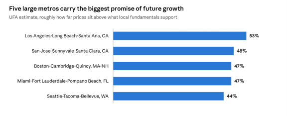
Which markets carry the biggest promise? UFA's estimates point to five large metros where prices sit roughly 44% to 53% above what local fundamentals support. These are the places with the most growth already built into the price, and the most to lose if it does not arrive.
The cost of owning
Property taxes and insurance premiums take a share of what owners pay each month. Every dollar a buyer spends on them is a dollar the buyer cannot bid into the price of the house. Rising carrying costs work like a small rise in interest rates: they lower what buyers can pay.
Property taxes also amplify the cycle. As we showed in Property Taxes Pour Fuel on the Housing Cycle, local governments set tax rates to meet revenue budgets. When values rise, rates tend to fall, which makes owning cheaper and pushes prices higher. When values fall, rates rise to protect revenue. Property taxes amplify booms and deepen busts.
What it means for mortgage risk
For lenders and investors, the promise in a house price is not abstract. It is the equity that protects a loan. When prices grow as expected, a borrower's equity builds year by year, and the loan becomes safer. When prices grow more slowly, that cushion builds more slowly. A loan that looks safe at origination stays exposed for longer.
This means today's loan-to-value ratios can overstate safety. They measure equity at today's price, and today's price assumes growth that may not arrive. Two loans with the same LTV and the same credit score can carry very different risk, depending on where the house sits.
The risk also has two horizons. In markets where supply has surged, it can arrive soon, through falling prices. In supply-constrained markets, it builds slowly, as the gap between promised and actual growth widens. A national view hides both. A house price is a bet on a place, and some places can't cover the bet.
A credit score asks whether the borrower can keep a promise. ForeScore asks the same of the place. It measures default and prepayment risk by ZIP code over the full life of a mortgage. Learn more about ForeScore or contact us.
Sources and data notes
- Survey of Consumer Expectations, © 2013–26 Federal Reserve Bank of New York (FRBNY). The SCE data are available without charge at www.newyorkfed.org and may be used subject to license terms posted there. FRBNY disclaims any responsibility or legal liability for this analysis and interpretation of Survey of Consumer Expectations data.
- S&P CoreLogic Case-Shiller U.S. National Home Price Index, not seasonally adjusted (CSUSHPINSA), via FRED.
- Congressional Budget Office, The Demographic Outlook: 2026 to 2056, January 2026
- Daniel McCue, Household and New Housing Unit Demand Projections for 2025–2035 and 2035–2045, Joint Center for Housing Studies of Harvard University, January 2025.
- John Mulford, The Income Elasticity of Housing Demand, RAND Corporation for HUD, 1979.
- DavidAlbouy, Gabriel Ehrlich and Yingyi Liu, Housing Demand, Cost-of-Living Inequality, and the Affordability Crisis, NBER Working Paper 22816
Timing note. Expectations are from each February survey. Actual appreciation is the change in the Case-Shiller national index over the following 12 months, February to February. Mortgage examples assume a fixed-rate 30-year loan.
-