Price models say prices revert to fundamental value but rarely define it. This paper draws on urban economics to supply that anchor.

‍

Abstract

Models of real estate price dynamics share a common structure. Prices carry recent changes forward and revert toward a fundamental value. Yet these models rarely say what that fundamental value is. They treat it as a statistical trend or estimate it from a few metropolitan aggregates. This paper argues that urban economics already supplies the missing anchor. Spatial equilibrium models explain why locations earn different rents. Growth models show that fundamental value includes the capitalized value of expected rent growth. Real-options models of irreversible development show that it also includes the value of waiting, and they explain why supply responds with a lag. Aggregating heterogeneous development options yields local supply elasticity, which in turn shapes the momentum and mean-reversion parameters of dynamic models. Quality-adjusted rent–price ratios provide an imperfect but disciplined way to observe the anchor. The synthesis clarifies what “overshooting” means, corrects a common intuition about when overshooting occurs, and yields testable predictions about how supply conditions affect the amplitude and duration of real estate cycles.

Keywords: fundamental value; urban land prices; real options; housing supply elasticity; price dynamics; mean reversion; rent–price ratio

JEL classification: R14, R31, R52, G12, D81

‍

1. Introduction

Why do real estate prices rise so much more in some places than in others? A positive demand shock in one metropolitan area may produce a building boom. The same shock elsewhere may produce soaring land prices and little new construction. In one market, appreciation fades as new supply arrives. In another, prices keep rising, attract attention, and may eventually overshoot the rents that support them.

A large empirical literature describes these patterns. House price changes are positively autocorrelated in the short run and mean-reverting in the long run (Case and Shiller 1989; Abraham and Hendershott 1996; Capozza, Hendershott, and Mack 2004). The workhorse model has two terms. One carries last period’s price change forward. The other pulls price back toward a fundamental value, usually written \(P^{*}\).

The second term raises a question the dynamic literature seldom answers: mean reversion to what? In most applications \(P^{*}\) is a statistical construct. It may be a trend, a cointegrating relation with income, or a cross-sectional regression on a few metropolitan fundamentals. Such constructs are useful. But without an economic definition of \(P^{*}\), we cannot say whether a price increase is capitalization of better fundamentals or a departure from them. A theory of overshooting requires a theory of what has been overshot.

This paper argues that urban economics supplies that theory. Three older literatures, usually read separately from the dynamics literature, together define the anchor and explain how prices move around it.

• Spatial equilibrium explains why locations earn different rents and why those rents are capitalized into land values (Alonso 1964; Mills 1967; Muth 1969; Rosen 1979; Roback 1982).

• Growth explains why fundamental value depends on the expected path of rents, not just their level (Arnott and Lewis 1979; Wheaton 1982; Capozza and Helsley 1989).

• Uncertainty and irreversibility explain why owners wait to develop, why undeveloped land carries option value, and why supply responds with a lag (Titman 1985; Williams 1991; Capozza and Helsley 1990; Capozza and Li 1994).

Aggregating development options across heterogeneous parcels yields local supply elasticity (Mayer and Somerville 2000; Saiz 2010). Supply elasticity, in turn, shapes the speed and amplitude of price adjustment (Glaeser, Gyourko, and Saiz 2008; Paciorek 2013). Finally, quality-adjusted rent–price ratios offer an empirical window on the otherwise unobserved anchor (Capozza and Seguin 1996; Campbell et al. 2009).

The central proposition is simple. Spatial fundamentals, growth, and option value determine the equilibrium toward which prices are anchored. Real-option considerations determine when supply responds. Local supply elasticity shapes the speed and amplitude of price adjustment around that equilibrium.

The paper is a synthesis, not a new model. Its contribution is to show how the pieces fit, to be precise about what \(P^{*}\)  contains, and to point out where the links have been asserted rather than derived. Section 2 sets out the spatial anchor. Section 3 adds growth, and Section 4 adds uncertainty and irreversibility. Section 5 aggregates options into supply. Section 6 turns to price dynamics and states exactly when overshooting occurs. Section 7 addresses measurement. Section 8 draws policy implications, and Section 9 concludes with open questions.

‍

2. Spatial Equilibrium: Where Fundamental Value Comes From

Every theory of price dynamics needs an anchor. For real estate, the anchor begins with location.

Two physically identical buildings can have very different values because one occupies a more valuable place. A building can be reproduced. A location cannot.

In the classic monocentric model, households and firms value access to a central business district. Commuting and transport costs generate differences in willingness to pay across space, and land rents capitalize those differences (Alonso 1964; Mills 1967; Muth 1969). Rents fall with distance from the center because occupants must be compensated for longer commutes.

Modern cities are more complicated. Employment is polycentric. Households value schools, amenities, safety, and access to many destinations. The Rosen–Roback framework generalizes the logic across cities: wages and rents adjust so that mobile households and firms are indifferent among locations (Rosen 1979; Roback 1982). Productivity and amenities are then capitalized into rents and land values. The underlying logic survives: location creates a stream of economic benefits, and land values capitalize that stream.

At its simplest, the asset value of a constant rent is
‍
\begin{equation}\label{eq:1}
P^{*} = \frac{R}{r}
\end{equation}
where \(R\) is the rent generated by the location and \(r\) is the discount rate. Growth, depreciation, taxes, risk, and redevelopment possibilities enrich the expression, but the economic idea remains.

The distinction between structures and land matters. Structures are reproducible; sites are not. Where new supply is easy to create, construction costs constrain the price of structures, and the residual value of location appears in land. That residual can arise from nature, infrastructure, agglomeration, amenities, or regulation (Glaeser and Gyourko 2018).

A demand shock changes the rent surface. Employment growth, a new transit line, or an improvement in amenities raises the value of occupying particular places. The shock does not begin with prices. It begins with a change in the economic value of location, which prices then capitalize.

More generally, the fundamental value of property \(i\) can be written
\begin{equation}\label{eq:2}
P_{i}^{*} = f\left( R_{i},g_{i},r_{i},X_{i} \right)
\end{equation}

where current rent, expected rent growth, required return, and other property and location characteristics jointly determine value. The next two sections show that \(f\) must include a growth premium and, for land that is not yet in its best use, an option premium.

Spatial equilibrium tells us where value is anchored. It does not yet tell us why asset prices can move well before current rents, why undeveloped land can command a premium, or why owners leave apparently profitable development opportunities unexercised. Those questions require us to introduce the future.

‍

3. Growth, Expectations, and the Price of Land

Location explains why rents differ across space. But current rent does not fully explain the price of land, because land is an asset and assets are priced for the future.

Consider two parcels that earn the same rent today. Rents on the first are expected to stay constant. Rents on the second are expected to rise as the city grows. The two parcels cannot have the same price. A buyer of the second parcel purchases not only today’s rent but also tomorrow’s higher rents.

Dynamic urban growth models formalize this idea (Arnott and Lewis 1979; Wheaton 1982). In the growing-city model of Capozza and Helsley (1989), the price of urban land decomposes into four parts: the value of agricultural rent, the cost of conversion, the value of accessibility, and the present value of expected future rent increases—a growth premium. Capozza and Schwann (1989) find empirical support for this asset approach to urban land.

3.1 The growth premium

Suppose rent is expected to rise by a constant amount \(g\)  per year, measured in dollars rather than as a percentage:
\begin{equation}\label{eq:3}
R(t + s) = R(t) + g\, s
\end{equation}

The value of the land is the discounted value of this rental stream:
\begin{equation}\label{eq:4}
P(t) = \int_{0}^{\infty}\left\lbrack R(t) + g\, s \right\rbrack e^{- rs}\, ds = \frac{R(t)}{r} + \frac{g}{r^{2}}
\end{equation}

The first term capitalizes current rent. The second is the growth premium.¹

A static capitalization model says price is proportional to current rent. A dynamic model says price depends on both the level of rent and its expected path. Growth can raise prices without raising current rents. Two cities with identical rents can have different land prices because one is expected to grow faster.

The two terms also differ in their sensitivity to discount rates. The elasticity of the current-rent term with respect to (r\) is \(- 1\). The elasticity of the growth premium is \(- 2\). The growth component therefore has roughly twice the duration of the current-rent component. Where much of value comes from expected growth — the share is \(g/(rR + g)\) —prices are especially sensitive to changes in interest rates and risk premiums. This helps explain why land prices, and prices in fast-growing markets, can move sharply even when current rents move little.

3.2 The city boundary

The growth premium is most visible at the urban fringe. Land just outside the city earns agricultural rent today, but its owner holds land that is expected to become urban. Its price incorporates the future rents associated with conversion. Land can acquire urban value before it acquires an urban use.

High fringe land prices therefore need not indicate speculation in the pejorative sense. They may reflect rational capitalization of anticipated growth. The market prices the city that is coming, not merely the city that exists.

3.3 Fundamentals include expectations

The growth model gives a richer definition of fundamental value:
\begin{equation}\label{eq:5}
P^{*} = \frac{R}{r} + \frac{g}{r^{2}}
\end{equation}

plus terms for conversion cost, alternative-use value, and accessibility. This is an important conceptual step. Discussions of real estate often contrast fundamentals with expectations, as though fundamentals describe the present and expectations are a departure from it. That cannot be right for a durable asset.

The relevant distinction is between expectations justified by the process that generates future rents and expectations that depart from that process. A theory of real estate prices is necessarily a theory of expectations.

3.4 From growth to development timing

If expected growth raises the value of land today, why does the owner not develop immediately? Growth tells us why the land is valuable. It does not tell us when the owner should convert it. Once development is irreversible and the future is uncertain, waiting itself has value.

‍

4. Uncertainty and the Value of Waiting

The growth argument assumed the future could be foreseen. Suppose instead that everyone expects a city to grow but no one knows how fast. A parcel that looks ready for development today may look much better tomorrow, or the growth may never come.

Uncertainty matters even when investors are risk-neutral. The reason is irreversibility. Once land has been converted, the decision cannot economically be undone. Before development, the owner holds something valuable: the right to wait. Titman (1985) and Williams (1991) established this option view of vacant land. Capozza and Helsley (1990) embedded it in a spatial equilibrium model of a growing city.

4.1 The development threshold

Let urban rent follow an arithmetic Brownian motion,
\begin{equation}\label{eq:6}
P^{*} = \frac{R}{r} + \frac{g}{r^{2}}
\end{equation}

where \(g\) is the expected growth in rent per year, \(\sigma\) is its volatility, and \(dz\) is the increment of a standard Wiener process. Let \(R_{A}\) be agricultural rent and \(C\) the cost of conversion. Define
\begin{equation}\label{eq:7}
\alpha = \frac{\sqrt{g^{2} + 2r\sigma^{2}} - g}{\sigma^{2}}
\end{equation}

which is the positive root of \(\frac{1}{2}\sigma^{2}\alpha^{2} + g\alpha - r = 0\). The owner converts when rent first reaches the hurdle
\begin{equation}\label{eq:8}
R^{*} = R_{A} + rC + \left( \frac{1}{\alpha} - \frac{g}{r} \right)
\end{equation}

This expression follows from value matching and smooth pasting.² The first two terms are the certainty hurdle: rent must cover the agricultural rent forgone and the interest on conversion cost. The term in parentheses is the premium for uncertainty, measured in dollars of rent. It is zero when \(\sigma = 0\), because \(\alpha\) then equals \(r/g\). It rises with \(\sigma\).

At the optimal conversion date, the conventional net present value of converting is positive. It equals \(1/(\alpha r)\). Part of this, \(g/r^{2}\), would be present even under certainty, because an owner facing rising rents gains by waiting for them. The rest, \((1/\alpha - g/r)/r\), is the price of flexibility under uncertainty. A positive NPV at the moment of development is therefore not evidence of irrational delay.

4.2 Uncertainty creates option value

Undeveloped land can sell for more than the capitalized value of its current use because its owner controls the timing of an irreversible investment. Growth and uncertainty create different premiums. Growth gives future urban use value. Uncertainty gives the timing decision value.
\begin{equation}\label{eq:9}
V_{\text{undeveloped}} = V_{\text{current use}} + V_{\text{development option}}
\end{equation}

Higher expected growth tends to bring development forward. Greater uncertainty tends to delay it. Capozza and Helsley (1990) show that uncertainty raises land values at the boundary above opportunity cost and reduces equilibrium city size. Capozza and Sick (1994) show that land awaiting conversion appreciates with rent growth and unsystematic risk, and that city size shrinks as systematic and unsystematic risk rise. Capozza and Li (1994, 2002) show that owners choose development intensity as well as timing, a result discussed further in Section 4.3. Grenadier (1996) shows that competition among owners can trigger development cascades and overbuilding.

The empirical evidence is broadly supportive. Quigg (1993) finds a measurable option premium in Seattle land prices. Capozza and Li (2001) find that residential investment responds to interest rates and volatility as the option model predicts. Cunningham (2006) finds that greater price uncertainty delays development and raises vacant land prices. Bulan, Mayer, and Somerville (2009) find that volatility delays condominium development, and that competition weakens the effect.

4.3 Density as a second margin: another value of waiting

Sections 4.1 and 4.2 treat development as a binary switch: land is either in agricultural use or converted, at a fixed built intensity, once rent crosses the hurdle R^*. Actual development decisions have a second margin. An owner who converts land also chooses how much to build on it---floor-area ratio, height, units per acre. That choice is made under the same uncertainty as the timing decision, and it is costly to reverse: adding density later typically requires substantial new investment, and building at low density when rent turns out to be high forecloses cheaply capturing the higher rent.

Capozza and Li (1994) model the landowner's problem as a joint choice of when to convert and how intensely to build. The result is not simply a different optimal density. It changes the value of undeveloped land itself. Because higher realized rent at the moment of conversion justifies, and elicits, denser development, the owner's payoff is a convex function of the rent path, not merely of whether rent has crossed a fixed threshold. Waiting is valuable for two reasons rather than one: it lets the owner pick the right time to develop, and it lets the owner discover the rent level to which the optimal density should respond. Equation (9) can be written more completely as
\[
V_{\text{development option}} = V_{\text{timing}} + V_{\text{intensity}}
\]

where \(V_{\text{timing}}\) is the option value already derived in Section 4.1 and \(V_{\text{intensity}}\) is the additional value that comes from being able to match the density of development to the rent realized when conversion occurs. Fixed-density models such as equation (8) implicitly set \(V_{\text{intensity}} = 0\): they hold the building program constant across states of the world and let only the date of conversion respond to rent.

Once intensity is allowed to respond as well, three results follow that fixed-density models cannot produce. First, land is worth more than fixed-density option models imply, for any given rent process, because the intensity margin adds a further convexity to the payoff. Second, the hurdle rent for conversion rises further above the certainty hurdle in equation (8), because the owner who waits captures not only a better price but also a better building. Third, the effect of the interest rate on development timing is not monotonic: a lower discount rate raises the value of the future flexibility to build denser, which can offset, and in some ranges reverse, the usual effect of lower rates in accelerating development. Capozza and Li (2002) extend the joint timing-intensity problem and derive the resulting optimal development rule; Capozza and Li (2001) find empirical support for interest-rate and volatility effects on residential investment consistent with this richer option structure. Amin and Capozza (1993) make a closely related point from a different angle: when development can proceed in stages rather than all at once, the owner holds a sequence of options, each exercised as rising rent justifies the next increment of building. The same logic that gives intensity choice its extra value gives sequential development its extra value---in both cases, the payoff responds to how much rent has risen, not only to whether it has crossed a threshold.

The practical implication for the anchor is that \(P^{*}\) for undeveloped or redevelopable land understates true fundamental value whenever it is built from a fixed-density option model. The gap is largest where zoning and construction technology allow a wide range of feasible densities, and smallest where density is effectively fixed by regulation or site constraints---in which case \(V_{\text{intensity}} \to 0\) and equation (8) is again the right benchmark. Section 5.1 returns to this point: the aggregation of options into supply below assumes fixed density for tractability, so the resulting supply curve should be read as a lower bound on the price sensitivity of density, not merely of the extensive margin of conversion.

4.4 What the anchor contains

The first three sections imply a precise definition. For a parcel in its best use, \(P^{*}\) is the capitalized value of current rent plus the growth premium, net of the risk adjustments embedded in \(r\). For land that is vacant or ripe for redevelopment, \(P^{*}\) also includes the value of the development option, now understood to include both the timing component of Section 4.1 and the intensity component of Section 4.3.  \(P^{*}\) moves whenever rents, expected growth, volatility, discount rates, or the feasible future use of land change.

This matters for any test of overshooting. If \(P^{*}\) omits the option premium, a rise in uncertainty that raises land values will look like a departure from fundamentals. It is not. The anchor itself has moved.

4.5 Prices move before construction

Prices can adjust immediately. Buildings cannot. Favorable news can raise land prices today while uncertainty keeps development options unexercised. A gap can therefore open between the speed of price adjustment and the speed of quantity adjustment. The next step is to aggregate individual options into a market supply response.

‍

5. From Options to Supply: Why Some Cities Build and Others Appreciate

A rise in demand has to go somewhere. It can produce more real estate or more expensive real estate. Usually it does both. The important question is how much of each.

A metropolitan market contains thousands of development options: vacant parcels, underused sites, redevelopment opportunities, additions, conversions, and changes in density. At any moment, a city holds a portfolio of unexercised options. The supply response to a demand shock depends on how easily those options can be exercised. That is supply elasticity.

5.1 Supply as aggregated option exercise

A positive demand shock raises rents and expected rents, so fundamental value rises. Higher prices move parcels toward their thresholds. Some cross them, and construction begins. Stock–flow models capture the lag between price signals and completed supply (DiPasquale and Wheaton 1994), and urban growth models can be used to estimate supply directly (Mayer and Somerville 2000).

The option model gives this aggregation a simple form. Suppose parcels differ only in conversion cost, with \(C_{j}\) distributed according to \(F\). Parcel \(j\) converts when rent reaches its own hurdle, \(R_{j}^{*} = R_{A} + rC_{j} + (1/\alpha - g/r)\). The share of parcels developed at rent \(R\) is then
\begin{equation}\label{eq:10}
S(R) = F\left( \frac{R - R_{A} - (1/\alpha - g/r)}{r} \right)
\end{equation}

This stylized expression has two useful implications. First, the density of \(F\) near the margin determines the local slope of supply: a market is elastic when many parcels sit just above the current hurdle. Second, volatility enters only through the uncertainty premium, which is common to all parcels. Higher \(\sigma\) therefore shifts the supply schedule to higher rents without changing its shape. By contrast, constraints that differ across parcels—remediation, parcel assembly, discretionary review—change the distribution \(F\) and therefore the shape of supply. The distinction is testable.

Allowing density to respond to rent, as in Section 4.3, adds an intensive margin that equation (10) does not capture. A rent increase then does two things at once: it converts additional parcels at the extensive margin, and it raises the built intensity of parcels already converted or now converting. Both margins add to measured supply elasticity, and a supply curve estimated from conversions alone, holding density fixed, will understate the full price responsiveness of a market where the intensive margin is available.

5.2 What makes an option expensive to exercise?

Some impediments are physical: water, steep terrain, or existing density. Some are technological: construction costs, infrastructure needs, or the jump to high-rise construction. Others are institutional: zoning, height limits, parking requirements, approval delays, and uncertainty about permission.

Saiz (2010) shows that metropolitan supply elasticities reflect both geography and regulation. Gyourko, Saiz, and Summers (2008) document large differences in regulation across markets. Some impediments raise conversion cost. Some add time. Some add uncertainty. Some remove development possibilities altogether. Their common effect is to weaken the quantity response to higher demand.

5.3 Elastic and inelastic markets

In an elastic market, higher prices induce conversion, redevelopment, and greater density. New supply absorbs part of the shock and eventually restrains rents and prices. In an inelastic market, the same shock raises rents and values but produces little construction. The shock stays capitalized in the existing stock, and prices do more of the adjusting.

Observed price growth is therefore not a pure measure of demand. It is the interaction of demand with the ability to create supply.

5.4 Supply as an arbitrage mechanism

In financial markets, traders perform arbitrage. In real estate, developers perform a form of real arbitrage by creating the asset. When existing space becomes expensive relative to the cost of producing new space, developers build, and new construction competes with the existing stock. This arbitrage is slow, costly, and irreversible, and in some places it is severely constrained. Its strength depends on the ability to build, which takes us from supply to price dynamics.

‍

6. Momentum, Mean Reversion, and the Dynamics of Price

Real estate prices have a peculiar memory. When prices rise this year, they often keep rising next year. But when prices move far from levels supported by fundamentals, they eventually come back (Case and Shiller 1989; Abraham and Hendershott 1996). In the short run, prices have momentum. In the long run, they mean-revert.

These facts are not contradictory. A demand shock changes fundamental value. Prices respond quickly; supply responds slowly. During the interval, recent price changes can persist. Eventually development, rents, and the limits set by fundamental value pull prices back.

6.1 A simple dynamic model

Following Capozza, Hendershott, and Mack (2004), write
\begin{equation}\label{eq:11}
\Delta P_{t + 1} = \phi\,\Delta P_{t} + \lambda\,\left( P_{t}^{*} - P_{t} \right) + \varepsilon_{t + 1}
\end{equation}

The parameter \(\phi\) measures momentum: how strongly recent changes carry forward. The parameter \(\lambda\) measures mean reversion: how strongly the gap between price and fundamental value is closed each period. Here \(P_{t}^{*}\) is the fundamental value of Sections 2–4. It includes the growth premium and, where relevant, option value. It is not a trend.

6.2 When does price overshoot?

A common intuition holds that overshooting occurs when momentum is strong relative to mean reversion. The precise condition is more interesting. The homogeneous part of equation (11) has characteristic equation
\begin{equation}\label{eq:12}
x^{2} - (1 + \phi - \lambda)\, x + \phi = 0
\end{equation}

The system is stable when \(0 \leq \phi < 1\) and \(0 < \lambda < 2(1 + \phi)\). Its roots are complex—so price oscillates around \(P^{*}\) —when
\begin{equation}\label{eq:13}
\left( 1 - \sqrt{\phi} \right)^{2} < \lambda < \left( 1 + \sqrt{\phi} \right)^{2}
\end{equation}

Three results follow.

1. Overshooting needs both forces. With \(\lambda = 0\) price never turns back. With \(\phi = 0\), price overshoots only if \(\lambda > 1\), which is implausible for annual data. Oscillation requires momentum and mean reversion together
   ‍
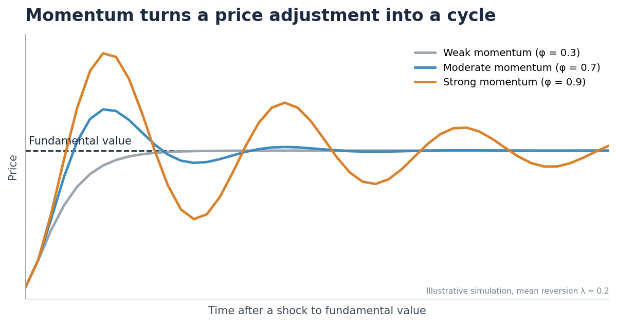
2. Momentum governs persistence. In the oscillatory region the roots have modulus \(\sqrt{\phi}\), so the amplitude of successive swings shrinks by a factor of \(\sqrt{\phi}\) each period regardless of \(\lambda\). With \(\phi = 0.9\), swings take about 13 periods to halve.
   ‍
3. Mean reversion governs timing and the initial overshoot. Holding \(\phi\) fixed, a larger \(\lambda\) shortens the cycle and, perhaps surprisingly, raises the first overshoot.

Table 1 illustrates these results. It shows the response of price to a permanent unit increase in \(P^{*}\), starting from equilibrium.

Table 1. Peak overshoot (percent of the change in \(P^{*}\)) and cycle length (periods)
‍

Note: Simulated from equation (11) with $\varepsilon = 0$. “None” means the roots are real and price approaches $P^{*}$ from below without overshooting. Half-life is the number of periods for the amplitude of swings to halve, $\ln 0.5/\ln\sqrt{\phi}$.
‍

The table shows why momentum is the dangerous parameter. Moving down a column raises the overshoot sharply and makes it last far longer. Moving across a row raises the overshoot more modestly and shortens the cycle. Capozza et al. (2002) find exactly this combination—high serial correlation and little mean reversion—in high-construction-cost metropolitan areas such as Boston, New York, San Francisco, Los Angeles, and San Diego, and conclude that substantial overshooting can occur there.

‍

6.3 Why prices have momentum

Two broad explanations exist, and they predict different things.

The first is rational friction. Real estate is heterogeneous and trades infrequently. Buyers and sellers search. Appraisals lean on recent comparable sales. Price discovery therefore takes time. Search and liquidity can generate momentum in a rational model (Head, Lloyd-Ellis, and Sun 2014), as can strategic complementarity in sellers’ list prices (Guren 2018).

The second is extrapolation. Buyers do not observe fundamental value. They observe rents, employment, construction, interest rates, and prices. If they read recent appreciation as news about future demand, willingness to pay rises, sellers raise reservation prices, and lenders see stronger collateral. Capozza and Seguin (1996) find evidence of such euphoria in U.S. housing markets. Glaeser and Nathanson (2017) show that buyers who partly extrapolate from past prices can generate momentum, overshooting, and mean reversion together.

The distinction matters because a purely rational spatial model struggles to produce observed momentum. Glaeser et al. (2014) find that a dynamic rational model in the Alonso–Rosen–Roback tradition matches mean reversion and much of price and construction volatility, but fails to match the strong year-to-year persistence of price changes. Frictions and extrapolation also differ in their predictions. Friction-based momentum should be larger where trading is thinner and properties more heterogeneous. Extrapolative momentum should be larger where recent appreciation has been high and where supply is slow to contradict it.

6.4 Supply determines whether momentum is disciplined

Supply elasticity plausibly affects both parameters. In an elastic city, appreciation induces construction. New supply becomes visible, vacancies rise, and rent growth moderates. Construction produces information that pushes against extrapolation, which should lower \(\phi\). Elastic supply also strengthens the correcting force, which should raise \(\lambda\).

These two effects do not work in the same direction on overshooting. Lower \(\phi\). reduces both the size and the persistence of overshooting. Higher \(\lambda\) shortens the cycle but, for given \(\phi\), raises the initial overshoot. The net effect is an empirical question. The evidence so far suggests the \(\phi\) channel dominates. Glaeser, Gyourko, and Saiz (2008) find that elastic markets have fewer and shorter price booms with smaller price increases, although they may overbuild more. Paciorek (2013) finds that regulation and geography amplify price volatility by lengthening permit lags and reducing the supply response.

Supply constraints need not create optimistic expectations. They allow those expectations to survive longer. Elastic supply disciplines beliefs with buildings.

6.5 The anatomy of a cycle

A boom need not begin as a bubble. Employment can grow, productivity can rise, interest rates can fall, and expected rents can increase. The rational price of real estate rises, and so does \(P^{*}\). The difficult question comes later: at what point does an increase justified by fundamentals become sustained by expectations of further increases? There need not be a sharp boundary. A boom can evolve continuously from capitalization into extrapolation.

To tell the two apart, we need an observable link between the asset price and the services the asset produces. That brings us back to rent.

‍

7. Rent, Price, and the Problem of Measuring Fundamentals

A theory of mispricing requires a measure of the right price. That is harder than it sounds. We observe transaction prices and, less well, rents. We observe interest rates, construction costs, employment, and income. We do not observe \(P^{*}\). Fundamental value is the discounted value of rents not yet realized, based on expectations that cannot be observed and discount rates that change over time.

Price alone cannot tell us whether a sharp increase reflects rising fundamentals or movement away from them. Rent is the natural place to look.

7.1 Price and rent

With a constant proportional growth rate \(\gamma\), the Gordon model gives
\begin{equation}\label{eq:14}
P = \frac{R}{r - \gamma}\quad \Rightarrow \quad\frac{R}{P} = r - \gamma
\end{equation}

For owner-occupied housing, the relevant comparison is the user cost of ownership, which adds property taxes, maintenance, depreciation, tax treatment, and a risk premium to the interest rate (Poterba 1984; Himmelberg, Mayer, and Sinai 2005). A low rent–price ratio can arise because required returns are low, expected growth is high, or both. A yield is not a thermometer that measures overvaluation directly. It is an equilibrium outcome.

The same problem arises over time. A falling yield can indicate excessive prices, but it can also reflect lower interest rates, lower risk premiums, or stronger expected rent growth. Campbell et al. (2009) decompose movements in the U.S. housing rent–price ratio into these components. Plazzi, Torous, and Valkanov (2010) show that commercial real estate cap rates forecast both returns and rent growth, with the balance varying across property types and markets.

7.2 Real estate is not a homogeneous asset

Buildings differ in age, location, lease structure, tenant quality, redevelopment potential, and risk. Pooling transactions into an average cap rate mixes these characteristics together. Changes in the composition of properties sold can then look like changes in pricing, even when the pricing rule has not changed. If we want to know whether investors are capitalizing higher expected growth, we cannot let variation in property characteristics masquerade as variation in expectations. We need a constant-quality yield.

7.3 Cleaning the yield

A hedonic yield regression takes the form
\begin{equation}\label{eq:15}
\left( \frac{R}{P} \right)_{it} = f\left( X_{it},M_{it},t \right) + u_{it}
\end{equation}

where \(X_{it}\) are property characteristics and \(M_{it}\) are market characteristics. The time component then captures changes in market pricing after observable differences in assets have been held constant. Regressions of this kind are well established for commercial cap rates (see, for example, Chervachidze and Wheaton 2013). Capozza and Seguin (1996) show that the predictive content of housing rent–price ratios depends on controlling for quality differences between rental and owner-occupied units. The raw yield describes transactions. The quality-adjusted yield describes pricing.

7.4 Prices make promises

Return to the growth model. A rise in expected growth raises price even if current rent does not change, so the current rent–price ratio falls. That is not evidence of mispricing. It is what the growth model predicts. But it raises a further question: did the expected growth arrive?

If the market correctly anticipated higher rents, later rent growth should validate the earlier price increase. If rents fail to materialize, the earlier increase needs another explanation. A high price relative to current rent is a statement about the future. Prices make promises, and the empirical task is to see whether the future keeps them.

A low yield does not identify a bubble. It identifies a question: what must investors believe for this price to be rational?

7.5 A measurement system for the theory

Rent measures the current value of occupying a property. Price measures the value of the expected stream of those services. The rent–price ratio measures how investors price current income relative to future income and required returns. Quality adjustment lets that ratio be compared across properties, markets, and time. Together these variables provide an imperfect but disciplined window on \(P^{*}\).

A claim that prices reflect higher expected growth must eventually confront rent growth. A claim that prices reflect permanently lower required returns must confront subsequent returns. A claim that prices have departed from fundamentals must explain why neither accounts for the divergence. The yield does not settle the argument. It organizes it.

8. Policy Implications: Prices, Supply, and the Cost of Delay

Governments affect what can be built, where, how densely, how quickly, with what infrastructure, and at what cost. These interventions can serve legitimate purposes. Development can impose congestion, environmental costs, fiscal burdens, and effects on neighbors. But regulation also changes prices. The framework clarifies how: policy affects not just the final quantity of development but the cost, timing, and uncertainty of option exercise.

8.1 The cost of regulation includes the cost of delay

Some regulations raise direct costs. Others operate through time. A project that needs years of uncertain approvals differs economically from an otherwise identical project that can start today. Delay postpones income and adds uncertainty about the conditions under which the option will be exercised. The relevant dimensions are cost, probability of approval, and time to decision. Paciorek (2013) finds that longer permit lags are a main channel through which regulation lowers supply elasticity and raises price volatility.

8.2 Predictability and permissiveness

A restrictive rule can at least be known. A discretionary process adds uncertainty about density, timing, conditions, and approval. Relaxing zoning reduces the constraint itself. Making approvals faster and more predictable reduces uncertainty about exercise. Both can increase supply responsiveness, through different channels.

The option framework warns that the effects of regulatory uncertainty are not one-sided. More uncertainty raises the exercise threshold and slows construction. But it also raises the option value of undeveloped land, so its effect on land prices is ambiguous. Its effect on the timing and elasticity of supply is not. The case for predictable approval rests on faster and more responsive supply, not on lower land values. How much predictability matters relative to permissiveness is an open empirical question.

8.3 Supply policy is also price-stabilization policy

Housing supply policy is usually discussed as an affordability issue. The dynamic model suggests a second reading: it is also a price-stability issue. When demand rises in an elastic market, construction absorbs part of the shock and changes the information facing market participants. Where construction is constrained, the corrective mechanism is weaker. This does not mean permissive land use eliminates cycles. Credit, interest rates, and macroeconomic shocks remain important. It means supply policy changes the transmission mechanism.

8.4 High prices are not, by themselves, evidence of bad policy

A productive or desirable city should be valuable. High wages, amenities, and strong expected growth can rationally command high land prices. The policy question is not simply why prices are high. It is why additional demand produces higher prices rather than more supply. Geography, technology, existing density, or policy may explain the answer, and only some of these can be changed.

8.5 Construction costs as a benchmark

Structures are reproducible; locations are not. Where new space can be supplied readily, prices should stay connected over long horizons to the cost of producing it. A persistent wedge between market prices and production costs deserves explanation (Glaeser and Gyourko 2018). It may reflect scarce land, amenities, external costs, or restrictions that prevent exercise. When market value far exceeds the cost of creating new space and development still does not occur, something is preventing exercise. The policy question is what.

8.6 Land-use and infrastructure policy

Land-use policy changes the value of existing land as well as future construction. Restrictions on competing supply capitalize scarcity into existing property. Expanding development rights creates value for the land that receives them while reducing scarcity rents elsewhere. Infrastructure works through the other side of the model. Transit, schools, flood protection, and utilities alter accessibility, amenities, risk, and the feasibility of development. They change \(P^{*}\) and may change the exercise value of development options. Policy evaluation should therefore ask not only how much can be built, but when, and with how much uncertainty.

‍

9. Conclusion: A Theory of Different Clocks

Real estate is about space. But real estate prices may be easier to understand as a problem of time.

The urban model begins with space. Locations differ in accessibility, amenities, productivity, and scarcity. Those differences generate rents, and rents are capitalized into land values. To understand why prices move, we must add the future. Expected growth raises value because ownership conveys a claim on rents that have not yet arrived. Uncertainty gives owners an option to wait. Supply therefore responds with a lag, and the lag differs across markets.

This gives real estate a distinctive temporal structure. Prices of listed real estate securities can change in minutes. Beliefs about local markets can shift in days. Property transactions reveal information over weeks and months. Rents adjust over months or years. Development takes years. The urban stock may take decades to change. These clocks are not synchronized.

9.1 The cycle as a race between clocks

A positive demand shock changes fundamental value because the expected stream of rents has changed. Asset prices respond quickly; the physical city cannot. During the interval, prices carry most of the adjustment. If information diffuses slowly or buyers extrapolate, momentum carries prices further. Eventually slower forces respond. Rents adjust, developers exercise options, construction arrives, and mean reversion begins. The real estate cycle is not simply a sequence of irrational departures from equilibrium. It is the observable result of economic processes that run at different speeds.

9.2 One framework

Spatial equilibrium explains where value comes from. Growth explains why value depends on where rents are going. Uncertainty and irreversibility explain why owners wait and what option value adds to the anchor. Aggregated option exercise explains supply elasticity. Momentum and mean reversion describe the path of prices around the anchor, and supply elasticity shapes both. Quality-adjusted yields help determine whether prices remain connected to the rents that support them. Policy influences nearly every link.

location → rent → expected growth and option value → fundamental value → option exercise → supply → price dynamics

Fundamental value is not fixed. It moves when rents, expected growth, volatility, discount rates, accessibility, or the feasible use of land change. A dynamic theory cannot treat every price increase as a departure from equilibrium, because sometimes the equilibrium itself is moving. The empirical challenge is to distinguish movement of the anchor from movement away from it.

9.3 Open questions

The synthesis also shows where the links remain asserted rather than derived. Four questions stand out.

1. From options to dynamics. Equation 10 links option exercise to supply, and equation 11 links supply to price dynamics only through reduced-form parameters. A model that derives \(\phi\) and \(\lambda\) from the distribution of exercise costs, approval delays, and volatility would close the chain.
   ‍
2. Which parameter does supply move? Section 6.4 argues that elasticity lowers \(\phi\) and raises \(\lambda\), with opposite effects on the initial overshoot. Metropolitan and tract-level elasticity estimates, combined with regulatory indexes, allow the two channels to be estimated separately.
   ‍
3. Does the anchor include option value in practice? Section 4.4 implies that measured \(P^{*}\) should rise with local volatility for land ripe for development. Tests of mean reversion that omit this term may mistake a moving anchor for mispricing.
   ‍
4. How much of measured supply elasticity is intensity, not conversion? Section 4.3 implies that part of a market' s price responsiveness operates through built density rather than through new parcels crossing the conversion threshold. Separating these two margins empirically would show how much of Section 5's supply elasticity equation 10 omit.

Demand can change without building anything. Supply cannot. A change in beliefs can immediately change the price of every property in a city, but changing the stock requires land, capital, approvals, construction, and time. The less a market can adjust in space, the more it must adjust in price. And the more slowly it adjusts in quantity, the longer that price adjustment can persist.

Real estate is fixed in space. Its economics unfolds through time.
‍

Footnotes

1. Throughout Sections 3--5, \(g\) denotes growth in rent \emph{levels} (dollars per year), which is also the drift of the arithmetic Brownian motion introduced in Section 4. Section 7 uses \(\gamma\) for a \emph{proportional} growth rate, as in the Gordon model.
   ‍
2. Developed land is worth \(R/r + g/r^{2} - C\). Undeveloped land is worth \(R_{A}/r + Be^{\alpha R}\). Setting the two values and their derivatives equal at \(R^{*}\) gives \(Be^{\alpha R^{*}} = 1/(\alpha r)\) and equation 8. The final term can also be written \((r - \alpha g)/(\alpha r)\), the form used in Capozza and Helsley (1990).

‍

References

Abraham, Jesse M., and Patric H. Hendershott. 1996. “Bubbles in Metropolitan Housing Markets.” Journal of Housing Research 7 (2): 191–207.

Alonso, William. 1964. Location and Land Use: Toward a General Theory of Land Rent. Cambridge, MA: Harvard University Press.

Amin, Kaushik, and Dennis R. Capozza. 1993. "Sequential Development." Journal of Urban Economics 34 (2): 142--158..

Arnott, Richard J., and Frank D. Lewis. 1979. “The Transition of Land to Urban Use.” Journal of Political Economy 87 (1): 161–169. https://doi.org/10.1086/260744.

Bulan, Laarni, Christopher Mayer, and C. Tsuriel Somerville. 2009. “Irreversible Investment, Real Options, and Competition: Evidence from Real Estate Development.” Journal of Urban Economics 65 (3): 237–251.

Campbell, Sean D., Morris A. Davis, Joshua Gallin, and Robert F. Martin. 2009. “What Moves Housing Markets: A Variance Decomposition of the Rent–Price Ratio.” Journal of Urban Economics 66 (2): 90–102.

Capozza, Dennis R., and Robert W. Helsley. 1989. “The Fundamentals of Land Prices and Urban Growth.” Journal of Urban Economics 26 (3): 295–306. https://doi.org/10.1016/0094-1190(89)90003-X.

Capozza, Dennis R., and Robert W. Helsley. 1990. “The Stochastic City.” Journal of Urban Economics 28 (2): 187–203. https://doi.org/10.1016/0094-1190(90)90050-W.

Capozza, Dennis R., Patric H. Hendershott, and Charlotte Mack. 2004. “An Anatomy of Price Dynamics in Illiquid Markets: Analysis and Evidence from Local Housing Markets.” Real Estate Economics 32 (1): 1–32. https://doi.org/10.1111/j.1080-8620.2004.00082.x.

Capozza, Dennis R., Patric H. Hendershott, Charlotte Mack, and Christopher J. Mayer. 2002. “Determinants of Real House Price Dynamics.” NBER Working Paper 9262.

Capozza, Dennis R., and Yuming Li. 1994. “The Intensity and Timing of Investment: The Case of Land.” American Economic Review 84 (4): 889–904.

Capozza, Dennis R., and Yuming Li. 2001. “Residential Investment and Interest Rates: An Empirical Test of Land Development as a Real Option.” Real Estate Economics 29 (3): 503–519. https://doi.org/10.1111/1080-8620.00020.

Capozza, Dennis R., and Yuming Li. 2002. “Optimal Land Development Decisions.” Journal of Urban Economics 51 (1): 123–142.

Capozza, Dennis R., and Gregory M. Schwann. 1989. “The Asset Approach to Pricing Urban Land: Empirical Evidence.” Real Estate Economics 17 (2): 161–174. https://doi.org/10.1111/1540-6229.00481.

Capozza, Dennis R., and Paul J. Seguin. 1996. “Expectations, Efficiency, and Euphoria in the Housing Market.” Regional Science and Urban Economics 26 (3–4): 369–386. https://doi.org/10.1016/0166-0462(95)02120-5.

Capozza, Dennis R., and Gordon A. Sick. 1994. “The Risk Structure of Land Markets.” Journal of Urban Economics 35 (3): 297–319. https://doi.org/10.1006/juec.1994.1018.

Case, Karl E., and Robert J. Shiller. 1989. “The Efficiency of the Market for Single-Family Homes.” American Economic Review 79 (1): 125–137.

Chervachidze, Serguei, and William C. Wheaton. 2013. “What Determined the Great Cap Rate Compression of 2000–2007, and the Dramatic Reversal during the 2008–2009 Financial Crisis?” Journal of Real Estate Finance and Economics 46 (2): 208–231. https://doi.org/10.1007/s11146-011-9334-z.

Cunningham, Christopher R. 2006. “House Price Uncertainty, Timing of Development, and Vacant Land Prices: Evidence for Real Options in Seattle.” Journal of Urban Economics 59 (1): 1–31.

DiPasquale, Denise, and William C. Wheaton. 1994. “Housing Market Dynamics and the Future of Housing Prices.” Journal of Urban Economics 35 (1): 1–27.

Glaeser, Edward L., and Joseph Gyourko. 2018. “The Economic Implications of Housing Supply.” Journal of Economic Perspectives 32 (1): 3–30. https://doi.org/10.1257/jep.32.1.3.

Glaeser, Edward L., Joseph Gyourko, Eduardo Morales, and Charles G. Nathanson. 2014. “Housing Dynamics: An Urban Approach.” Journal of Urban Economics 81: 45–56.

Glaeser, Edward L., Joseph Gyourko, and Albert Saiz. 2008. “Housing Supply and Housing Bubbles.” Journal of Urban Economics 64 (2): 198–217.

Glaeser, Edward L., and Charles G. Nathanson. 2017. “An Extrapolative Model of House Price Dynamics.” Journal of Financial Economics 126 (1): 147–170.

Grenadier, Steven R. 1996. “The Strategic Exercise of Options: Development Cascades and Overbuilding in Real Estate Markets.” Journal of Finance 51 (5): 1653–1679.

Guren, Adam M. 2018. “House Price Momentum and Strategic Complementarity.” Journal of Political Economy 126 (3): 1172–1218. https://doi.org/10.1086/697207.

Gyourko, Joseph, Albert Saiz, and Anita A. Summers. 2008. “A New Measure of the Local Regulatory Environment for Housing Markets: The Wharton Residential Land Use Regulatory Index.” Urban Studies 45 (3): 693–729. https://doi.org/10.1177/0042098007087341.

Head, Allen, Huw Lloyd-Ellis, and Hongfei Sun. 2014. “Search, Liquidity, and the Dynamics of House Prices and Construction.” American Economic Review 104 (4): 1172–1210. https://doi.org/10.1257/aer.104.4.1172.

Himmelberg, Charles, Christopher Mayer, and Todd Sinai. 2005. “Assessing High House Prices: Bubbles, Fundamentals and Misperceptions.” Journal of Economic Perspectives 19 (4): 67–92.

Mayer, Christopher J., and C. Tsuriel Somerville. 2000. “Residential Construction: Using the Urban Growth Model to Estimate Housing Supply.” Journal of Urban Economics 48 (1): 85–109.

Mills, Edwin S. 1967. “An Aggregative Model of Resource Allocation in a Metropolitan Area.” American Economic Review 57 (2): 197–210.

Muth, Richard F. 1969. Cities and Housing: The Spatial Pattern of Urban Residential Land Use. Chicago: University of Chicago Press.

Paciorek, Andrew. 2013. “Supply Constraints and Housing Market Dynamics.” Journal of Urban Economics 77: 11–26.

Plazzi, Alberto, Walter Torous, and Rossen Valkanov. 2010. “Expected Returns and Expected Growth in Rents of Commercial Real Estate.” Review of Financial Studies 23 (9): 3469–3519.

Poterba, James M. 1984. “Tax Subsidies to Owner-Occupied Housing: An Asset-Market Approach.” Quarterly Journal of Economics 99 (4): 729–752.

Quigg, Laura. 1993. “Empirical Testing of Real Option-Pricing Models.” Journal of Finance 48 (2): 621–640.

Roback, Jennifer. 1982. “Wages, Rents, and the Quality of Life.” Journal of Political Economy 90 (6): 1257–1278.

Rosen, Sherwin. 1979. “Wage-Based Indexes of Urban Quality of Life.” In Current Issues in Urban Economics, edited by Peter Mieszkowski and Mahlon Straszheim, 74–104. Baltimore: Johns Hopkins University Press.

Saiz, Albert. 2010. “The Geographic Determinants of Housing Supply.” Quarterly Journal of Economics 125 (3): 1253–1296. https://doi.org/10.1162/qjec.2010.125.3.1253.

Titman, Sheridan. 1985. “Urban Land Prices under Uncertainty.” American Economic Review 75 (3): 505–514.

Wheaton, William C. 1982. “Urban Residential Growth under Perfect Foresight.” Journal of Urban Economics 12 (1): 1–21.

Williams, Joseph T. 1991. “Real Estate Development as an Option.” Journal of Real Estate Finance and Economics 4 (2): 191–208.

‍

‍